.jpg)
Developing a project for identifying the forest fire and wildfire system is an alternatively good example to exhibit one’s skills in Data Science. The forest fire or wildfire is an uncontrollable fire that develops in a forest. All the forest fir will create havoc during weekends on the animal habitat, surrounding environment and human property. k-means clustering can be used for the identification of the crucial hotspots during forest fire and to reduce the severity , to regulate them and even to predict the behaviour of the wildfire. This is advantageous for allocating the required resources. To enhance the model’s accuracy, it is ideal to use climatological data to find out the common periods and seasons for wildfires.
In this example, we develop a classification method for predicting forest fires.
This is a project, since the variable to be predicted is binary (fire or not fire).
The goal here is to model the probability of a fire occurring according to the day, month, certain meteorological variables, and a series of indices developed by the FWI system.
The comprises a data matrix in which columns represent variables, and rows represent instances.
The data file contains the information for creating the model. Here, the number of variables is 9, and the number of instances is 515.
This data set contains the following whose contain data measured in the northeast region of Portugal:
The total number of is 515. They are divided into training, generalization, and testing subsets. The number of training instances is 333 (80%), the number of selection instances is 45 (10%), and the number of testing instances is 45 (10%).
Once the data set has been set, we can perform a few related analytics. First, we check the provided information and ensure that the data has good quality.
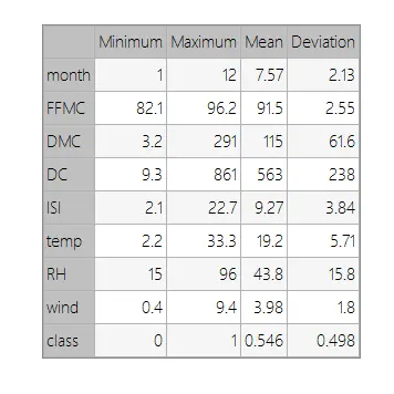
We can calculate the data statistics and draw a table with the minimums, maximums, means, and standard deviations of all variables in the data set. The following table depicts the values.
Also, we can calculate the for all variables. The following figure shows a pie chart with the proportion of fire (positives) and not fire (negatives) following our dataset.
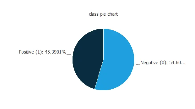
As we can see, the number of fire cases is 45.4% of the samples, and not fire represents approximately 54.6% of the pieces.
Finally, the might indicate to us what factors most influence fires.
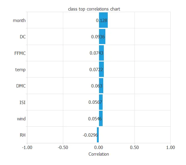
Here, the different variables are little correlated. Indeed, forest fire depends on many factors at the same time.
The second step is to set to represent the classification function. For this class of applications, the neural network is composed of:
The contains the statistics on the inputs calculated from the data file and the method for scaling the input variables. Here the minimum and maximum methods have been set. Nevertheless, the mean and standard deviation methods would produce very similar results.
The number of is 1. This perceptron layer has 8 inputs and 8 neurons.
Finally, we will set the for the as we want the predicted target variable to be binary.
The following picture shows a graph of the neural network for this example.
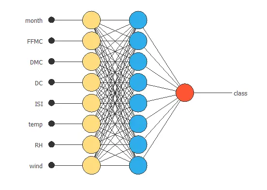
The yellow circles represent scaling neurons, the blue circles perceptron neurons, and the red circles probabilistic neurons. The number of inputs is 8, and the number of outputs is 1.
The procedure used to carry out the learning process is called a The training strategy is applied to the neural network to obtain the best possible performance. The type of training is determined by how the adjustment of the parameters in the neural network takes place. This process is composed of two terms:
The that we use is the with This is the default loss index for binary classification applications.
The learning problem is finding a neural network that minimizes the loss index. That is, a neural network that fits the data set and does not oscillate.
The that we use is the This is also the standard optimization algorithm for this type of problem.
The following chart shows how the error decreases with the iterations during the training process.
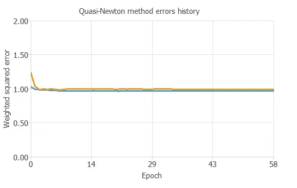
The final training and selection errors are training error = 0.966 WSE and selection error = 0.933 WSE, respectively.
The objective of is to find the network architecture with the best generalization properties, that is, that which minimizes the error on the of the data set.
More specifically, we want to find a neural network with a selection error of less than 0.933 WSE, which is the value that we have achieved so far. algorithms train several network architectures with a different number of neurons and select that with the smallest selection error.
The method starts with a small number of neurons and increases the complexity at each iteration.
The last step is to test the generalization performance of the trained neural network.
The objective of the is to validate the generalization performance of the trained neural network. To validate a classification technique, we need to compare the values provided by this technique to the observed values. We can use the as it is the standard testing method for binary classification projects.
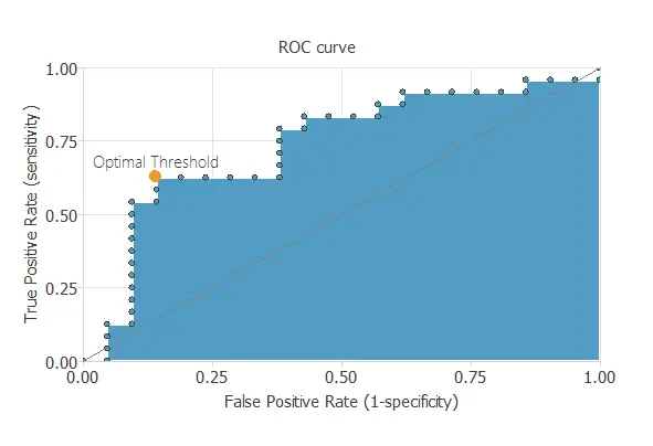
In the rows represent the target classes and the columns the output classes for the testing target data set. The diagonal cells in each table show the number of correctly classified cases, and the off-diagonal cells show the misclassified instances.
The following table shows the confusion elements for this application. The following table contains the elements of the confusion matrix.
| Predicted positive | Predicted negative | |
|---|---|---|
| Real positive | 13 (28.9%) | 8 (18.7%) |
| Real negative | 7 (15.6%) | 17 (37.8%) |
As we can see, the number of instances that the model can correctly predict is 30 (66.7%), while it misclassifies 15 (33.3%).
The next list depicts the for this application:
The neural network is now ready to predict outputs for inputs that it has never seen.
Below, a specific prediction having determined values for the model's input variables is shown.
The model predicts that the previous values correspond to a probability of fire is about 74%.
We objective of the response optimization algorithm is to exploit the mathematical model to look for optimal operating conditions.
Indeed, the predictive model allows us to simulate different operating scenarios and adjust the control variables to improve efficiency.
An example is to minimize fire probability in a fixed month.
The next table resumes the conditions for this problem.
| Variable name | Condition | |
|---|---|---|
| Month | Equal to | 9 |
| FFMC | None | |
| DMC | None | |
| ISI | None | |
| Temperature | None | |
| RH | None | |
| Wind speed | None | |
| Fire probability | Minimize |
The next list shows the optimum values for previous conditions.
The represented by the neural network, which can be exported to any specific software, is written below.
scaled_month = month*(1+1)/(12-(1))-1*(1+1)/(12-1)-1;
scaled_FFMC = FFMC*(1+1)/(96.19999695-(82.09999847))-82.09999847*(1+1)/(96.19999695-82.09999847)-1;
scaled_DMC = DMC*(1+1)/(291.2999878-(3.200000048))-3.200000048*(1+1)/(291.2999878-3.200000048)-1;
scaled_DC = DC*(1+1)/(860.5999756-(9.300000191))-9.300000191*(1+1)/(860.5999756-9.300000191)-1;
scaled_ISI = ISI*(1+1)/(22.70000076-(2.099999905))-2.099999905*(1+1)/(22.70000076-2.099999905)-1;
scaled_temp = temp*(1+1)/(33.29999924-(2.200000048))-2.200000048*(1+1)/(33.29999924-2.200000048)-1;
scaled_RH = RH*(1+1)/(96-(15))-15*(1+1)/(96-15)-1;
scaled_wind = wind*(1+1)/(9.399999619-(0.400000006))-0.400000006*(1+1)/(9.399999619-0.400000006)-1;

perceptron_layer_0_output_0 = logistic[ 0.595337 + (scaled_month*0.365295)+ (scaled_FFMC*-0.421814)+ (scaled_DMC*0.666443)+ (scaled_DC*0.126282)+ (scaled_ISI*-0.1427)+ (scaled_temp*0.479919)+ (scaled_RH*-0.277588)+ (scaled_wind*-0.0090332) ];
perceptron_layer_0_output_1 = logistic[ 0.745605 + (scaled_month*0.215881)+ (scaled_FFMC*0.39386)+ (scaled_DMC*0.468689)+ (scaled_DC*-0.083252)+ (scaled_ISI*-0.942017)+ (scaled_temp*0.669189)+ (scaled_RH*-0.74292)+ (scaled_wind*0.649841) ];
perceptron_layer_0_output_2 = logistic[ 0.490295 + (scaled_month*-0.260254)+ (scaled_FFMC*-0.546326)+ (scaled_DMC*-0.00305176)+ (scaled_DC*0.404602)+ (scaled_ISI*0.790894)+ (scaled_temp*0.639038)+ (scaled_RH*-0.43158)+ (scaled_wind*-0.126587) ];
perceptron_layer_0_output_3 = logistic[ -0.0189209 + (scaled_month*-0.864746)+ (scaled_FFMC*-0.548584)+ (scaled_DMC*-0.697632)+ (scaled_DC*-0.962402)+ (scaled_ISI*-0.0921631)+ (scaled_temp*0.247986)+ (scaled_RH*-0.161255)+ (scaled_wind*-0.158508) ];
perceptron_layer_0_output_4 = logistic[ 0.399719 + (scaled_month*0.683105)+ (scaled_FFMC*-0.915894)+ (scaled_DMC*-0.323242)+ (scaled_DC*-0.207825)+ (scaled_ISI*0.925049)+ (scaled_temp*0.611633)+ (scaled_RH*0.728943)+ (scaled_wind*0.547729) ];
perceptron_layer_0_output_5 = logistic[ 0.274475 + (scaled_month*0.472839)+ (scaled_FFMC*-0.127686)+ (scaled_DMC*-0.808655)+ (scaled_DC*0.556091)+ (scaled_ISI*-0.12561)+ (scaled_temp*0.547974)+ (scaled_RH*-0.957092)+ (scaled_wind*-0.192749) ];
perceptron_layer_0_output_6 = logistic[ 0.846924 + (scaled_month*0.379395)+ (scaled_FFMC*0.230347)+ (scaled_DMC*0.486023)+ (scaled_DC*-0.238708)+ (scaled_ISI*0.405518)+ (scaled_temp*0.272766)+ (scaled_RH*0.641235)+ (scaled_wind*0.514526) ];
perceptron_layer_0_output_7 = logistic[ 0.772766 + (scaled_month*0.289612)+ (scaled_FFMC*0.786621)+ (scaled_DMC*0.808289)+ (scaled_DC*0.266663)+ (scaled_ISI*0.136658)+ (scaled_temp*0.344666)+ (scaled_RH*-0.394348)+ (scaled_wind*-0.848816) ];

    probabilistic_layer_combinations_0 = 0.578857 +0.953979*perceptron_layer_0_output_0 +0.302429*perceptron_layer_0_output_1 +0.491089*perceptron_layer_0_output_2 -0.742981*perceptron_layer_0_output_3 -0.139282*perceptron_layer_0_output_4 -0.347168*perceptron_layer_0_output_5 -0.456177*perceptron_layer_0_output_6 +0.837708*perceptron_layer_0_output_7

class = 1.0/(1.0 + exp(-probabilistic_layer_combinations_0);


logistic(x){
   return 1/(1+exp(-x))
}
With the previous algorithm created (the mathematical expression), we can predict the fire risk and generate a fire map risk. The following images show an example of such a map:
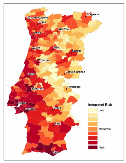
The image above shows the Portugal forest fire risk.
Note : Find the best solution for electronics components and technical projects ideas
keep in touch with our social media links as mentioned below
Mifratech websites : https://www.mifratech.com/public/
Mifratech facebook : https://www.facebook.com/mifratech.lab
mifratech instagram : https://www.instagram.com/mifratech/
mifratech twitter account : https://twitter.com/mifratech
Contact for more information : [email protected] / 080-73744810 / 9972364704